Experiments


The 140 page “PS-15 Experimental Manual” describes more than two dozen experiments to teach NMR at different levels.
Each section of the manual provides introductory information about the subject, specifies the problem and gives detailed instructions on conducting the experiment.
All of these experiments have been performed using an off-the-shelf PS15 NMR spectrometer and only originally acquired data are presented.
The PS-15 Experimental manual includes more than two dozen basic and advanced experiments. In addition there are several experiments on instrumentation.
Teachers and students have the freedom to use the samples provided or to select their own samples to use with the described sequences.
Acquired data can be manipulated with the tools on the data acquisition page, or if binary data is exported in ASCII format, users can use their own software to perform Fast Fourier Transform or calculate relaxation times.

PS-15 Experiments Included in the Experimental Manual
- Spectrometer “dead time”
- Spin-lattice relaxation (T1) measurements by:
- Inversion Recovery,
- Saturation Recovery
- Spin-spin relaxation (T2) measurements by:
- Spectrum line width
- Hahn spin-echo
- Carr-Purcell (CP)
- Car-Purcell-Meiboom-Gill (CPMG)
Basic experiments
- Obtaining on- and off-resonance Free Induction Decay (FID)
- Determining Π/2, Π, 3/2Π, etc pulses
- Phase adjustment for spectrometer phase sensitive detector
- Fast Fourier Transform of FID signal
- Comparison of liquid- and solid-like samples by NMR
- Two-exponential FID in wood and polymers
- Obtaining on and off-resonance spin-echo
- Rotating magnetization along different axis of reference frame
- Signal-to-Noise measurements
Instrumentation experiments
- Mapping the probehead RF coil
- Watching pulse sequence with an oscilloscope
- Amplitude detector versus phase sensitive detector
- Properties of lambda-quarter cable
Advanced experiments
- Angle dependence of spectra in the gypsum monocrystal
- Rotating frame experiments
- Multiple echoes with three pulse sequence

Examples of Experimental Results

NMR spectra: Liquids and solids
Liquids and solids present two extreme cases for NMR spectroscopy.
Liquids permit the movement of molecules that consequently average internal magnetic dipole-dipole interactions. If not averaged, the dipole-dipole interactions can generate a locally additional magnetic field in the vicinity of the nucleus under investigation which will modify the constant magnetic field B0. Thus NMR lines from liquid-like samples are usually very narrow.
On the other hand the rigid structure of solids limits the freedom of molecular motion preventing time averaging of local interactions and therefore produces a local magnetic field. This internal field is responsible for the dramatic broadening of the spectrum.
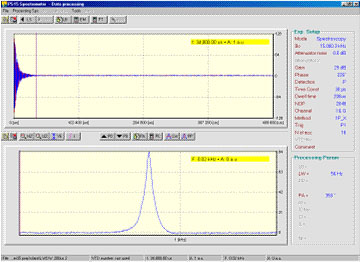
FID and spectrum from water doped with CuSO4. Note that FID is very long (almost 35 µs) and the spectrum line width (line width at half height) is only 56 Hz, typical for liquid-like samples. Natural line width is much narrower; here it is broadened by magnet inhomogeneity. (Click image to enlarge)

FID and spectrum from acrylic sample. Note that FID lasts less than 50 µs and the line width is very large, (25,000 Hz), typical for solid-like samples. (Click image to enlarge)
Wood
Some substances display properties of both liquids and solids. Wood is a good illustration of this case. It contains free, mobile water in capillaries and bound, highly rigid water. The free (liquid-like) water is responsible for the long component in FID signal, whereas bound water (solid-like) for its short component. After Fourier transform, free water is responsible for the narrow peak and bound water for the wide part of the spectrum.

Two-exponential decay of FID and narrow- and wide component of NMR spectrum in wood.

Relaxation Experiments

T1 measurements by IR method in glycerin; processing experimental data.
T1 spin-lattice relaxation in glycerin
At the equilibrium state all nuclear moments in a sample are distributed among the energy levels according to Boltzmann’s law.
The Boltzmann distribution slightly prefers an orientation of nuclear moments towards the polarizing field B0. This preference builds a minute nuclear macroscopic magnetization M0 along the B0 field. Following any process which disrupts this distribution, eg applying RF pulses, the nuclear spin system returns to equilibrium with the surrounding lattice by a process called spin-lattice relaxation that is characterized by a time T1.
Pulse NMR provides the most versatile method to measure T1 relaxation times over a wide range of times. PS15 software supports two popular methods of T1,measurements:
- Inversion Recovery method
- Saturation Recovery method
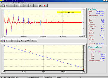
T2 measurement in glycerin by Carr-Purcell method. Due to inaccuracy of adjustment of the Πx pulse length echo-train contains only 16 echoes.
T2 spin-spin relaxation in glycerin
Spin-spin relaxation time describes processes that are responsible for bringing nuclear spins to an equilibrium state with each other after being exciting by an RF pulse.
Due to this process, spins loose their coherence. As a consequence a dephasing of the movement of nuclear spins takes place.
PS15 spectrometer supports four methods for T2 measurements:

T2 measurement in glycerin by Carr-Purcell-Meiboom-Gill method. Note that as many as 22 echoes are visible for T2 calculations.
- Signal width at half maximum
- Hahn two pulse sequence
- Carr-Purcell (CP)
- Carr-Purcell-Meiboom-Gill (CPMG)
The last three methods are based on the fact that dephasing of nuclear spins due to magnetic field inhomogeneity is reversible under certain conditions. This allows the measurement of intrinsic spin-spin T2 relaxation time. The Hahn method is relatively long and is sensitive for nuclear diffusion. The Carr-Purcell method suffers from possible cumulative errors that originate from the inaccuracy of the adjustment of RF pulse length. Modified by Meiboom and Gill, the CP method ingeniously circumvents the aforementioned problems.

Advanced Experiments

Rotating Frame Experiments
The rotating coordinate frame is a convenient reference frame for use in analyzing the interaction of the macroscopic nuclear magnetization M0, arising from the polarization of individual nuclear spins in the static magnetic field B0, with the rotating magnetic field B1. In the rotating frame that moves with the B1 field, nuclear spins are stationary, or in the presence of static field inhomegeneity, they move very slowly. Since the laws of Physics are independent of the reference frame, this slow motion of spins in the rotating frame implies that the effective magnetic field in the rotating frame must be much smaller than in a laboratory frame (or zero when the spins do not move at all).
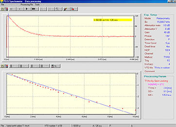
Spin locking experiment in rubber. With varied locking time one can measure T1ρ.
“Spin-locking” is one experiment illustrating the benefits of multiple power sequences with independently adjusted time, phase and power of the individual pulses. This feature, available only on commercial spectrometers, is available also in the PS15 spectrometer.
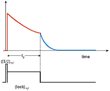
A “Spin-locking” sequence consists of two RF pulses. First is a short Π/2 pulse along the +x axis that moves the magnetization M0 on the x’y’ plane. Soon after the Π/2 pulse is completed, a second much longer RF pulse along the +y axis is applied. If B1 >> ΔB0 magnetization My and field M0 are parallel so there is no torque exerted on My and magnetization is “spin-locked” to B1. The longitudinal relaxation process that follows along B1 is somewhat similar to spin-lattice relaxation along B0 and is called T1 in the rotating frame characterized by a T1ρ. Since in a rotating frame the magnetization is polarized in a much smaller field (B1<<B0) the magnetization needs to relax from My=M0 to the much smaller equilibrium value. When the locking pulse ends the magnetization, the x’y’ plane inevitably decays very quickly due to spin-spin relaxation (blue line).

Multiple Echoes In Three Pulse Sequence
In his classic paper “Spin Echoes” (Phys. Rev. 80, 589-594, 1950), E. Hahn introduced the concept of pulsed NMR and an idea of Π/2 pulses.
He was so attached to the rotation of nuclear magnetization by 90 degrees that even the first nuclear spin-echo, which he called a product of “constructive interference” were generated by sequence of three Π/2 pulses.

Formation of multiple echoes in distilled water by (Π/2-τ-Π/2-TD-Π/2) sequence: Π/2=3.μs, τ=10ms, TD=25ms, repetition time TR=10s

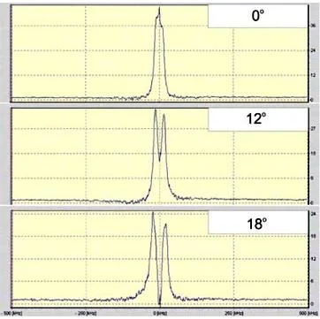
Angle Dependence of Spectra Shape in the Gypsum Monocrystal
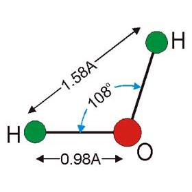
Atoms distances and angle in a water molecule according to Pake. H-H distance of 1.58??was calculated from spectra splitting. H-O distance was calculated from assumption of 108o angle of H-O-H bond.
It has been seen from the study of oriented crystals, that 1H NMR spectra of solid samples can give structural information that X-ray crystallography cannot deliver due to poor X-ray scattering on the hydrogen single electron.
This observation was first published by G. E. Pake (Journal of Chemical Physics vol.16, p327-336, 1948, “Nuclear Resonance Absorption in Hydrated Crystals: Fine Structure of the Proton Line”) in the early years of NMR. He observed the splitting of the NMR line from water protons in a hydrated gypsum (CaSO4·H20) monocrystal and powdered samples. The splitting originates from the interacting of magnetic dipoles μ in a static magnetic field B0. In crystalline solids these interactions produce an additional local magnetic field B1oc which contributes to the effective magnetic field acting on each spin. In less rigid substances, (mostly gases and liquids) fast molecular motion averages this local magnetic field to zero.

Gypsum monocrystal
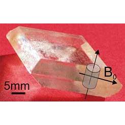
Sample cut from gypsum monocrystal and its orientation with regard to external magnetic field B0.

Gypsum crystal assembly in the magnet.
Sample cut from gypsum monocrystal and its orientation with regard to external magnetic field B0.

Instrumentation Experiments

Probehead RF Coil Mapping
To observe nuclear magnetic resonance phenomenon, the nuclei precessing around a constant magnetic field B0 must be exposed on the radio frequency field B0 that rotates in the plane perpendicular to the B0 field.
This rotating field, or circularly polarized field, of magnitude B1 can be obtained from the decomposition of a linearly oscillating field (linearly polarized) of magnitude 2B1. Only the field component that rotates in coherence with the precessing nuclear magnetization is used. The other one is radiated in space and lost.
In experimental practice the linearly polarized B1 field can be easily produced by a single closed loop driven by source of high frequency electromotive force.
The homogeneity of a B1 field generated by a single loop is rather poor. It can by improved by combining a series of single loops into a solenoid. The solenoid incorporated into the probehead resonance circuit is the most popular kind of transmit/receive antenna used in pulsed NMR spectroscopy. Its high homogeneity remains an important issue in experiments that require precisely defined rotating angles (Carr-Purcell). One can address B1 field homogeneity by reducing the sample volume but it has its limit due to degradation of S/N ratio.

Decomposition of linearly polarized field into two circular fields.

Single loop driven by a source of Electromotive Force (a) and solenoid b) as a source of linearly polarized field B1.
Instructions to measure B1 field distribution along the solenoid longitudinal axis
- Connect experimental setup
- Place the pick-up coil in the RF coil center
- Load one-pulse 1P_X method and set transmitter attenuation for 12dB, pulse width for 50μs and repetition time for 300ms
- On the oscilloscope get stable triggering by an external pulse and adjust vertical gain to see bottom and top part of the pulse
- Move pickup coil up and down and record the peak-to-peak amplitude of the pulse and the corresponding pickup coil position
- Repeat measurements until the amplitude of the pulse drops to about of 1% of its peak value
- With spreadsheet program (e.g.Excel) make a plot of the intensity of the RF pulse versus pickup coil position
- Find the position of the maximum signal and the area of its 10% drop. Consider this area as most useful in terms of B1 homogeneity. Mark it on the sample positioner and use as reference in your experiments. For fine experiments like CP and CPMG try to reduce size of the sample to the value you have obtained (3mm in this example).

Experimental setup to map the B1 intensity inside the RF coil and to monitor RF pulses. a) Pick-up coil inside the RF coil, b) pickup coil holder, c) linearly polarized B1 field within the solenoid.

Intensity of signal induced in the pickup coil vs. its position relative to the upper edge of probehead sample holder

"Magic Cable" or Properties of Lambda-Quarter Cable

Passive T/R switch diagram
The PS 15, as with many other contemporary pulsed NMR spectrometers, uses a single resonance circuit for generating an oscillating B1 field and for the reception of the precessing nuclear signal.
There is a conflict of applying power pulses from the transmitter to the resonance circuit and the simultaneous protection of the sensitive preamplifier connected to the same resonator. An electronic device called a multiplexer or transmit/receive switch (T/R) switches the resonance circuit between the transmitter and the preamplifier. The multiplexer must operate at a high frequency, switch very fast, withstand the high power of RF pulses and not introduce any losses or distortion to the nuclear signal.
The PS15 multiplexer design is based on the impedance transforming properties of the coaxial cable of a length corresponding to 1/4 of the electromagnetic wave length λ (1/4λ) at the frequency of interest and of the nonlinear properties of crossed semiconductor diodes connected antiparallel.
Generally for a coaxial cable length of any odd number of quarters of wavelength,

the input impedance of the cable is described by the formula

where Z0 is cable impedance and ZL is loading impedance.

When grounded on one end (ZL=0) the cable shows infinite input impedance, while the input impedance of the unloaded cable drops to zero.
After loading the cable with an impedance of ZL=Z0 the input impedance becomes the cable’s characteristic impedance Z0.
The wavelength of an electromagnetic wave in vacuum is given by

where c is speed of light in a vacuum, and f is the electromagnetic wave frequency. Assuming c=3x10^9 m/s and f=15x10^6 Hz (15 MHz) we can estimate the lambda quarter length as 5 m. In a coaxial cable, however, there is no vacuum but there is the dielectric isolator so the speed of the electromagnetic wave is much slower than 3x10^9 m/s, thus λ/4 is considerably shorter. With an RG 174/U coaxial cable a quarter lambda line is about 3.3 meters.
Due to their strong nonlinear voltage-current dependence, a semiconductor diode shows high impedance properties for low voltages, and low impedance properties for high voltages. Therefore diodes operate like a switch which is open for large signals and closed for small signals. Two antiparallel connected crossed diodes combine these properties for positive as well for negative voltages and can operate also as the aforementioned switch for an alternating signal. For silicon diodes this switching point is around 0.7 V.

If combined together a λ/4 cable and two sets of crossed semiconductor diodes will work as a tricky transmit/receive switch described below.
Transmit period:
- Both crossed diodes D1 and D2 conduct during RF power pulses (high voltage opens diodes). As a consequence the transmitter is connected to the resonance circuit while the preamplifier is disconnected from the dangerously overloaded resonance circuit.

Receive period:
- Immediately after the RF pulse is turned off, the impedance of diodes D1 and D2 increase (the low voltage case where diodes do not conduct). This closes the path through the D1 diodes from the transmitter to the resonance circuit isolating it from the noise coming from the transmitter’s direction. Meanwhile the high impedance of diodes D2 opens the λ/4 coax cable and connects the resonator to the preamplifier.

To show “magic” properties of the λ/4 cable we will conduct a simple experiment by connecting the cable to the output of the preamplifier and shorten and “un-shorten” the cable with a piece of wire while observing the FID signal on the data display.
Instructions
· Plug a BNC T-type adapter between the probehead RX output (this is a preamplifier output) and the unit RX input (this is receiver input).
· On the setup page prepare a one-pulse experiment with the glycerin sample.
· Connect opened λ/4 cable to the T adapter. Note the drop of signal on the setup data window
· Now shorten the coax cable output with the BNC jack or a piece of wire and pair of crocodile clips to ground. Note signal recovery on the setup data window. Conclusion
As you see one can not apply common sense to results obtained with a λ/4 cable operating at 15 MHz. Under certain conditions the coaxial cable works as a unique impedance transformer that transforms a low load impedance to a high input impedance (or high load to low input impedance).
Experimental setup
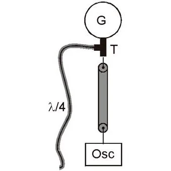
More Experiments with λ/4 cable
If you have a signal generator (G) and an oscilloscope (Osc) available in your laboratory you can make a more systematic study of λ/4 cable properties. Connect an experimental setup as shown and change the frequency of the generator with the λ/4 shorted to ground. Look for the maximum of the signal at 15 MHz. Now open the cable, change the frequency and observe the minimum of the signal at 15 MHz.
Connect an additional piece of coax cable through the BNC barrel adapter and look at the shift of frequency of the maximum/minimum signal toward lower frequencies.
You can replace the oscilloscope with more advanced device like a network analyzer and have the cable frequency characteristics in a matter of seconds.
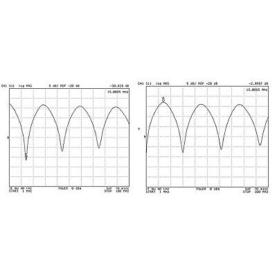
Reflected power from λ/4 15 MHz cable. Left- cable shorted to ground
